Rapid computation and visualisation of convective parameters from rawinsonde and numerical weather prediction data
thundeR is a freeware R package for rapid computation and visualisation of convective parameters commonly used in the operational forecasting of severe convective storms. Core algorithm is based on C++ code implemented into R language via Rcpp. This solution allows to compute over 200 thermodynamic and kinematic parameters in less than 0.02s per profile and process large datasets such as reanalyses or operational NWP models in a reasonable amount of time. Package has been developed since 2017 by research meteorologists specializing in severe convective storms and is constantly updated with new features.
Online browser
Online rawinsonde browser of thundeR package is available at http://rawinsonde.com
Installation
The stable version can be installed from the CRAN repository:
install.packages("thunder")The development version can be installed directly from the github repository:
remotes::install_github("bczernecki/thunder")Usage
Draw Skew-T, hodograph and convective parameters on a single layout and export to png file
data("sounding_vienna") # load example dataset (Vienna rawinsonde profile for 23 Aug 2011 12UTC):
pressure = sounding_vienna$pressure # vector of pressure [hPa]
altitude = sounding_vienna$altitude # vector of altitude [meters]
temp = sounding_vienna$temp  # vector of temperature [degree Celsius]
dpt = sounding_vienna$dpt # vector of dew point temperature [degree Celsius]
wd = sounding_vienna$wd # vector of wind direction [azimuth in degrees]
ws = sounding_vienna$ws # vector of wind speed [knots]
sounding_save(filename = "Vienna.png", title = "Vienna - 23 August 2011 1200 UTC", pressure, altitude, temp, dpt, wd, ws)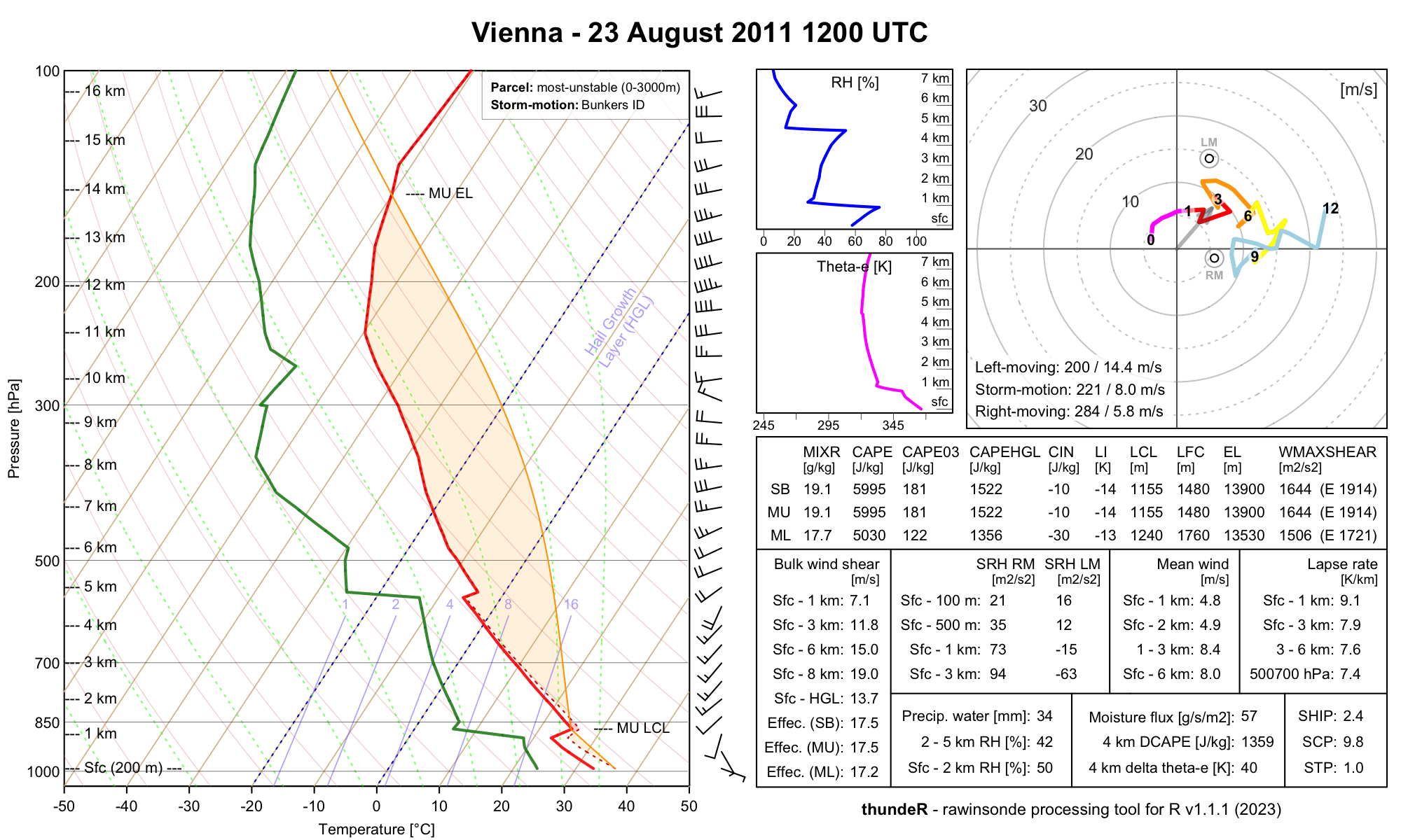
Download LBF North Platte rawinsonde profile for 03 Jul 1999 00UTC and export to png file
profile = get_sounding(wmo_id = 72562, yy = 1999, mm = 7, dd = 3, hh = 0)

sounding_save(filename = "NorthPlatte.png", title = "North Platte - 03 July 1999 0000 UTC", profile$pressure, profile$altitude, profile$temp, profile$dpt, profile$wd, profile$ws)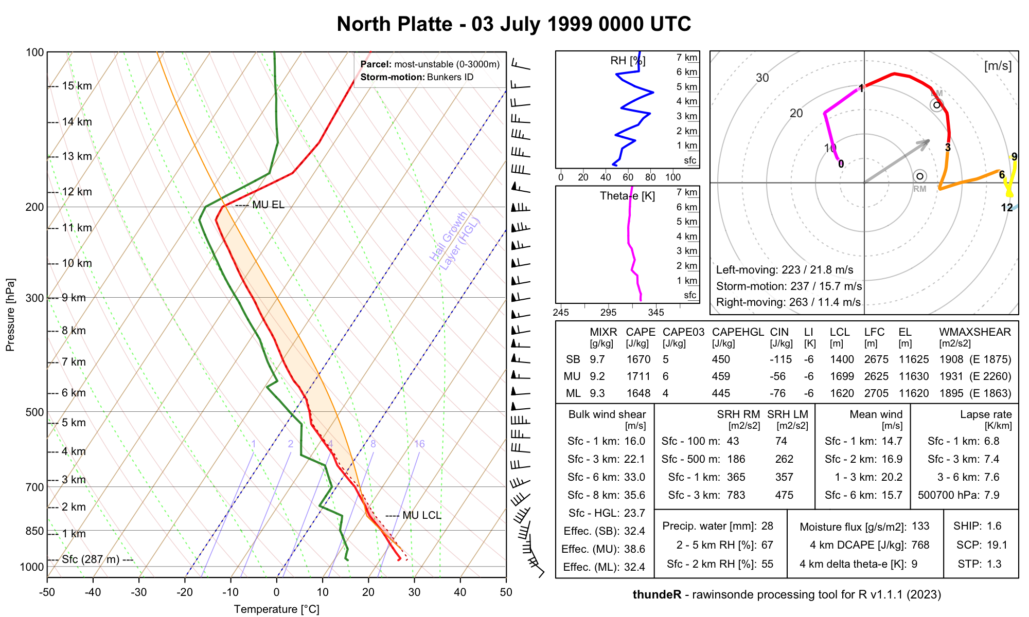
Compute convective parameters based on a sample vertical profile data:
library("thunder")

pressure = c(1000, 855, 700, 500, 300, 100, 10) # pressure [hPa]
altitude = c(0, 1500, 2500, 6000, 8500, 12000, 25000) # altitude [meters]
temp = c(25, 10, 0, -15, -30, -50, -92) # temperature [degree Celsius]
dpt = c(20, 5, -5, -30, -55, -80, -99) # dew point temperature [degree Celsius]
wd = c(0, 90, 135, 180, 270, 350, 0) # wind direction [azimuth in degress]
ws = c(5, 10, 20, 30, 40, 5, 0) # wind speed [knots]
accuracy = 2 # accuracy of computations where 3 = high (slow), 2 = medium (recommended), 1 = low (fast)
sounding_compute(pressure, altitude, temp, dpt, wd, ws, accuracy)


#              MU_CAPE          MU_CAPE_M10       MU_CAPE_M10_PT         MU_02km_CAPE
#            2269.9257             998.1443             313.0747             247.9794
#         MU_03km_CAPE          MU_HGL_CAPE               MU_CIN           MU_LCL_HGT
#             575.6293            1616.5384               0.0000             730.0000
#           MU_LFC_HGT            MU_EL_HGT                MU_LI            MU_LI_M10
#             730.0000            8300.0000             -10.1119             -10.8539
#              MU_WMAX           MU_EL_TEMP          MU_LCL_TEMP          MU_LFC_TEMP
#              67.3784             -28.8000              17.7000              17.7000
#              MU_MIXR          MU_CAPE_500      MU_CAPE_500_M10   MU_CAPE_500_M10_PT
#              14.8759            1076.0322             389.3651             137.0814
#           MU_CIN_500            MU_LI_500        MU_LI_500_M10              SB_CAPE
#               0.0000              -5.0417              -6.2346            2269.9257
#          SB_CAPE_M10       SB_CAPE_M10_PT         SB_02km_CAPE         SB_03km_CAPE
#             998.1443             313.0747             247.9794             575.6293
#          SB_HGL_CAPE               SB_CIN           SB_LCL_HGT           SB_LFC_HGT
#            1616.5384               0.0000             730.0000             730.0000
#            SB_EL_HGT                SB_LI            SB_LI_M10              SB_WMAX
#            8300.0000             -10.1119             -10.8539              67.3784
#           SB_EL_TEMP          SB_LCL_TEMP          SB_LFC_TEMP              SB_MIXR
#             -28.8000              17.7000              17.7000              14.8759
#              ML_CAPE          ML_CAPE_M10       ML_CAPE_M10_PT         ML_02km_CAPE
#            1646.0639             670.1001             225.2816             164.0798
#         ML_03km_CAPE          ML_HGL_CAPE               ML_CIN           ML_LCL_HGT
#             422.4290            1250.0221               0.0000             975.0000
#           ML_LFC_HGT            ML_EL_HGT                ML_LI            ML_LI_M10
#             975.0000            7900.0000              -7.6203              -8.5845
#              ML_WMAX           ML_EL_TEMP          ML_LCL_TEMP          ML_LFC_TEMP
#              57.3771             -26.4000              15.2500              15.2500
#              ML_MIXR             LR_0500m              LR_01km              LR_02km
#              13.0487             -10.0000             -10.0000             -10.0000
#              LR_03km              LR_04km              LR_06km              LR_16km
#              -9.0476              -7.8571              -6.6667              -6.0000
#              LR_26km              LR_24km              LR_36km          LR_26km_MAX
#              -5.0000              -5.7672              -4.2857              -5.7143
#         LR_500700hPa         LR_500800hPa         LR_600800hPa             FRZG_HGT
#              -4.2857              -5.1807              -5.8333            2500.0000
#     FRZG_wetbulb_HGT  HGT_max_thetae_03km  HGT_min_thetae_04km         Delta_thetae
#            2275.0000               0.0000            3750.0000              28.0698
# Delta_thetae_min04km          Thetae_01km          Thetae_02km                DCAPE
#              28.8346             330.5323             323.6191             598.3100
#   Cold_Pool_Strength           Wind_Index           PRCP_WATER   Moisture_Flux_02km
#              12.6322              33.9064              27.1046              30.4255
#              RH_01km              RH_02km              RH_14km              RH_25km
#               0.7291               0.7197               0.6452               0.5550
#              RH_36km               RH_HGL             BS_0500m              BS_01km
#               0.4436               0.4603               1.9172               3.8344
#              BS_02km              BS_03km              BS_06km              BS_08km
#               8.7821              12.6560              18.0055              17.4077
#              BS_36km              BS_26km              BS_16km              BS_18km
#               9.3693              13.3304              16.6478              20.2791
#            BS_EFF_MU            BS_EFF_SB            BS_EFF_ML        BS_SFC_to_M10
#              14.2232              14.2232              13.8968              15.5104
#        BS_1km_to_M10        BS_2km_to_M10     BS_MU_LFC_to_M10     BS_SB_LFC_to_M10
#              13.6499               9.8830              14.0737              14.0737
#     BS_ML_LFC_to_M10        BS_MW02_to_SM        BS_MW02_to_RM        BS_MW02_to_LM
#              13.6864               7.3040              10.1410              10.7870
#         BS_HGL_to_SM         BS_HGL_to_RM         BS_HGL_to_LM             MW_0500m
#               4.8934               7.7860               9.9885               2.3086
#              MW_01km              MW_02km              MW_03km              MW_06km
#               2.4251               3.3476               4.8003               7.8107
#              MW_13km          SRH_100m_RM          SRH_250m_RM          SRH_500m_RM
#               6.8389               4.2535              10.0537              19.7206
#           SRH_1km_RM           SRH_3km_RM          SRH_36km_RM          SRH_100m_LM
#              39.6346             152.5219             236.5901               1.5027
#          SRH_250m_LM          SRH_500m_LM           SRH_1km_LM           SRH_3km_LM
#               3.5518               6.9670              14.0023             -13.1308
#          SRH_36km_LM           SV_500m_RM           SV_01km_RM           SV_03km_RM
#             -24.3790               0.0039               0.0039               0.0048
#           SV_500m_LM           SV_01km_LM           SV_03km_LM        MW_SR_500m_RM
#               0.0010               0.0011              -0.0014              10.0863
#        MW_SR_01km_RM        MW_SR_03km_RM        MW_SR_500m_LM        MW_SR_01km_LM
#              10.1501               9.5359              13.7821              12.8585
#        MW_SR_03km_LM     MW_SR_VM_500m_RM     MW_SR_VM_01km_RM     MW_SR_VM_03km_RM
#               8.4579              10.1078              10.2253              10.5358
#     MW_SR_VM_500m_LM     MW_SR_VM_01km_LM     MW_SR_VM_03km_LM       SV_FRA_500m_RM
#              13.7647              12.8371               8.8342               0.9982
#       SV_FRA_01km_RM       SV_FRA_03km_RM       SV_FRA_500m_LM       SV_FRA_01km_LM
#               0.9871               0.9560               0.2592               0.2800
#       SV_FRA_03km_LM         Bunkers_RM_A         Bunkers_RM_M         Bunkers_LM_A
#              -0.2862             209.4046               7.7933             122.0585
#         Bunkers_LM_M         Bunkers_MW_A         Bunkers_MW_M   Corfidi_downwind_A
#              13.1825             151.9494               7.8107             218.6955
#   Corfidi_downwind_M     Corfidi_upwind_A     Corfidi_upwind_M              K_Index
#              14.6982             231.3283               9.1794              24.3548
#      Showalter_Index    TotalTotals_Index          SWEAT_Index              STP_fix
#               3.7501              44.3548             106.4168               0.3600
#              STP_new           STP_fix_LM           STP_new_LM              SCP_fix
#               0.2005               0.1272               0.0708               6.2338
#              SCP_new           SCP_fix_LM           SCP_new_LM                 SHIP
#               4.9243              -0.5367              -0.4239               0.6287
#                  HSI                  DCP         MU_WMAXSHEAR         SB_WMAXSHEAR
#               1.7159               1.1507            1213.1848            1213.1848
#         ML_WMAXSHEAR     MU_EFF_WMAXSHEAR     SB_EFF_WMAXSHEAR     ML_EFF_WMAXSHEAR
#            1033.1051             958.3359             958.3359             797.3548
#             EHI_500m             EHI_01km             EHI_03km          EHI_500m_LM
#               0.2798               0.5623               2.1638               0.0988
#          EHI_01km_LM          EHI_03km_LM              SHERBS3               SHERBE
#               0.1987              -0.1863               0.6482               0.7015
#           SHERBS3_v2            SHERBE_v2                  DEI              DEI_eff
#               0.8642               0.9353               1.5198               1.1885
#                  TIP
#               2.4356
Hodograph example:
Download sounding and draw hodograph:
data("northplatte")
sounding_hodograph(ws = northplatte$ws, wd = northplatte$wd, altitude = northplatte$altitude, max_speed = 38)
title("North Platte - 03 July 1999, 00:00 UTC")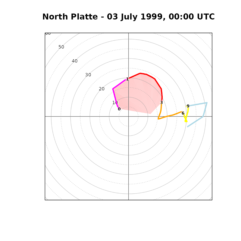
Perform sounding computations using Python with rpy2:
It is possible to launch thunder under Python via rpy2 library. Below you can find the minimum reproducible example:
Make sure that pandas and rpy2 libraries are available for your Python environment. If not install required python packages:
Launch thunder under Python with rpy2:
# load required packages
from rpy2.robjects.packages import importr
from rpy2.robjects import r,pandas2ri
import rpy2.robjects as robjects
pandas2ri.activate()

# load thunder package (make sure that it was installed in R before)
importr('thunder')

# download North Platte sounding
profile = robjects.r['get_sounding'](wmo_id = 72562, yy = 1999, mm = 7, dd = 3,hh = 0)

# compute convective parameters
parameters = robjects.r['sounding_compute'](profile['pressure'], profile['altitude'], profile['temp'], profile['dpt'], profile['wd'], profile['ws'], accuracy = 2)


# customize output and print all computed variables, e.g. most-unstable CAPE (first element) equals 9413 J/kg

print(list(map('{:.2f}'.format, parameters)))
['9413.29', '233.35', '1713.74', '0.00', '775.00', '775.00',
'15500.00', '-16.55', '137.21', '-66.63', '23.98', '23.98',
'23.36', '9413.29', '233.35', '1713.74', '0.00', '775.00',
'775.00', '15500.00', '-16.55', '137.21', '-66.63', '23.98',
'23.98', '23.36', '7805.13', '115.22', '1515.81', '-4.35',
'950.00', '950.00', '15000.00', ...]
Accuracy tables for sounding_compute()
The interpolation algorithm used in the sounding_compute() function impacts accuracy of parameters such as CAPE or CIN and the performance of the script. The valid options for the accuracy parameter are 1, 2 or 3:
accuracy = 1 - High performance but low accuracy. Dedicated for large dataset when output data needs to be quickly available (e.g. operational numerical weather models). This option is around 20 times faster than high accuracy (3) setting. Interpolation is peformed for 60 levels (m AGL):
c(0, 100, 200, 300, 400, 500, 600, 700, 800, 900, 1000, 1100, 1200, 1300, 1400, 1600, 1800, 2000, 2200, 2400, 2600, 2800, 3000, 3200, 3400, 3600, 3800, 4000, 4200, 4400, 4600, 4800, 5000, 5200, 5400, 5600, 5800, 6000, 6500, 7000, 7500, 8000, 8500, 9000, 9500, 10000, 10500, 11000, 11500, 12000, 12500, 13000, 13500, 14000, 15000, 16000, 17000, 18000, 19000, 20000)accuracy = 2 - Compromise between script performance and accuracy. Recommended for efficient processing of large numerical weather prediction datasets such as meteorological reanalyses for research studies. This option is around 10 times faster than high accuracy (3) setting. Interpolation is peformed for 318 levels (m AGL):
c(0, 10, 20, 30, 40, 50, 60, 70, 80, 90, 100, 110, 120, 130, 140, 150, 160, 170, 180, 190, 200, 210, 220, 230, 240, 250, 260, 270, 280, 290, 300, 310, 320, 330, 340, 350, 360, 370, 380, 390, 400, 410, 420, 430, 440, 450, 460, 470, 480, 490, 500, 510, 520, 530, 540, 550, 560, 570, 580, 590, 600, 610, 620, 630, 640, 650, 660, 670, 680, 690, 700, 710, 720, 730, 740, 750, 775, 800, 825, 850, 875, 900, 925, 950, 975, 1000, 1025, 1050, 1075, 1100, 1125, 1150, 1175, 1200, 1225, 1250, 1275, 1300, 1325, 1350, 1375, 1400, 1425, 1450, 1475, 1500, 1525, 1550, 1575, 1600, 1625, 1650, 1675, 1700, 1725, 1750, 1775, 1800, 1825, 1850, 1875, 1900, 1925, 1950, 1975, 2000, 2025, 2050, 2075, 2100, 2125, 2150, 2175, 2200, 2225, 2250, 2275, 2300, 2325, 2350, 2375, 2400, 2425, 2450, 2475, 2500, 2525, 2550, 2575, 2600, 2625, 2650, 2675, 2700, 2725, 2750, 2775, 2800, 2825, 2850, 2875, 2900, 2925, 2950, 2975, 3000, 3050, 3100, 3150, 3200, 3250, 3300, 3350, 3400, 3450, 3500, 3550, 3600, 3650, 3700, 3750, 3800, 3850, 3900, 3950, 4000, 4050, 4100, 4150, 4200, 4250, 4300, 4350, 4400, 4450, 4500, 4550, 4600, 4650, 4700, 4750, 4800, 4850, 4900, 4950, 5000, 5050, 5100, 5150, 5200, 5250, 5300, 5350, 5400, 5450, 5500, 5550, 5600, 5650, 5700, 5750, 5800, 5850, 5900, 5950, 6000, 6100, 6200, 6300, 6400, 6500, 6600, 6700, 6800, 6900, 7000, 7100, 7200, 7300, 7400, 7500, 7600, 7700, 7800, 7900, 8000, 8100, 8200, 8300, 8400, 8500, 8600, 8700, 8800, 8900, 9000, 9100, 9200, 9300, 9400, 9500, 9600, 9700, 9800, 9900, 10000, 10100, 10200, 10300, 10400, 10500, 10600, 10700, 10800, 10900, 11000, 11100, 11200, 11300, 11400, 11500, 11600, 11700, 11800, 11900, 12000, 12250, 12500, 12750, 13000, 13250, 13500, 13750, 14000, 14250, 14500, 14750, 15000, 15250, 15500, 15750, 16000, 16250, 16500, 16750, 17000, 17250, 17500, 17750, 18000, 18250, 18500, 18750, 19000, 19250, 19500, 19750, 20000)accuracy = 3: High accuracy but low performance setting. Recommended for analysing individual profiles. Interpolation is performed with 5 m vertical resolution step up to 20 km AGL (i.e.: 0, 5, 10, ... 20000 m AGL)
Important notes
- Remember to always input wind speed data in knots.
- Script will always consider first height level as the surface (h = 0), therefore input height data can be as above sea level (ASL) or above ground level (AGL).
- For efficiency purposes it is highly recommended to clip input data for a maximum of 16-18 km AGL or lower.
- Values of parameters will be different for different accuracy settings.
Developers
thundeR package has been developed by atmospheric scientists, each having an equal contribution (listed in alphabetical order):
Bartosz Czernecki (Adam Mickiewicz University in Poznań, Poland)
Piotr Szuster (Cracow University of Technology, Poland)
Mateusz Taszarek (CIMMS/NSSL in Norman, Oklahoma, United States)